Singapore Flat Price Predictor

Predict Singapore Flat Price with machine learning

Singapore has been chosen as one of the most expensive country by The Economist Intelligence Unit for the fifth year in a row. As one of the most expensive cities in the world, accommodation constitutes a very big part of the expenses.

In order to provide affordable housing for the general population in Singapore, Singapore government has been offering some public housing options in Singapore, more generally known as the HDB Flat.

For this side project, I have taken the HDB Resale Prices data and trained a machine learning model to predict the flat resale price of Singapore.

In line with the Smart Nation initiative, Singapore government has published a lot of Singapore data online and it is publicly available to access. Moreover, there are some nice APIs available for the developers to integrate with their application.

Overview

The article is broken down into few sections. Below is an overview of the sections that I am covering:

1. Visualize the data
2. Feature Creation
3. Train/Test Splitting
4. Experiment
5. Create Machine Learning model
6. Ensemble
7. Metrics
8. Results
9. Conclusion

Without further ado, let’s dive in and see how to create a flat price predictor yourself !

Visualize the data

Before starting in a machine learning project, it is important that we carry out some standard visualization procedures to understand our data. Only by understanding our data, we would know the right approach in cleaning and preprocessing our data.

Below are the available columns in this data:

'month', 'town', 'flat_type', 'block', 'street_name', 'storey_range', 'floor_area_sqm', 'flat_model', 'lease_commence_date', 'resale_price'

Resale price would be the target label in this project, and the rest of the columns will form our feature matrix. Let’s go on and plot some graph.

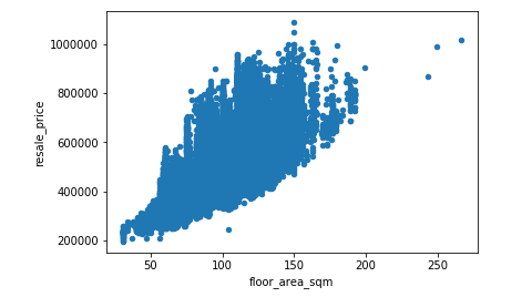
We can infer from this graph that, the higher the floor area, the higher is the resale price of of the flat. By plotting distribution graph, we can spot if there are any outliers and remove them if they look too unusual.

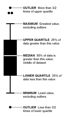
Besides that, we can also use boxplot to understand the distribution of our data. Below is a simple diagram of boxplot, and it is helpful in showing us the distribution of the target label given a particular feature.

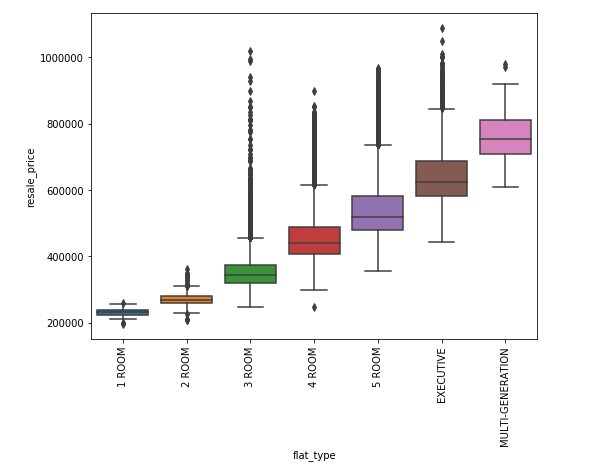
In the context of our project, boxplot can help us understand the distribution of the flat price among different flat type.

Another important visualization that will help us understanding our features would be the correlation matrix:

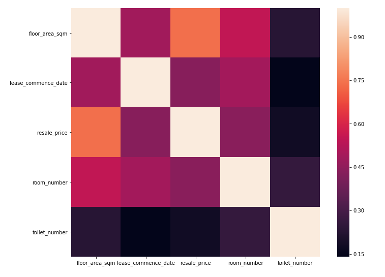
So what is the takeaway from this matrix? The color between floor area and the resale price are the lightest among other combinations. It means that floor area and resale price are highly correlated in a positive way — higher floor area, higher resale price.

In contrast, toilet number and resale price have very low correlation, which means toilet number might not be very useful in predicting the resale price of the flat.

Feature Creation

The features that are available in this data set are considerably small. But, nothing stop us from creating more!

Having more features is definitely going to help the machine learning model to learn the patterns of this data set.

Some of the features that I think will be useful:

1. Direction. The town where the flat is located is given in this data set. How could we improve on this feature? I create a new feature, that map the town to one of the direction/region listed below:

"NORTH_EAST","EAST""WEST","NORTH","CENTRAL"

2. Room number & toilet number. Based on the flat type that is given, I check from the HDB website and find out the number of rooms and toilets and create two more new features.

3. Storey. The storey range features provided in the data is in a string format: 4 TO 6, 7 TO 9, which I think is sub-optimal because if your features are ordinal, you should convert the feature to number.

The reason being, floor 7 is lower than floor 9, and modeling the feature as number will help the model to learn this relationship. If we leave the feature as string without any processing, the model will miss out this great information.

So I create a random generator that will generate a number between the lowest storey and highest storey given in the dataset. Look at the example below to understand better:

# Example, :
4 To 6 - The generator output: 4 or 5 or 6
7 TO 9 - The generator output: 7 or 8 or 9

4. Sales Year & Month. The month originally given in the data set are in this format: 2018–4, so by breaking them up to ‘year’ and ‘month’ will allow the model to pick up the ordinal relationship.

How effective are the newly created features in improving our model’s performance? I will be running multiple experiments and do some comparison with the base model. I will cover that in the later section of Results.

Train/Test Splitting

We would need to split our data into train and test set to validate the accuracy of our model before we actually push this model into production. Something important to note when creating our train test set:

1. The distribution of train and test set should be similar. A bad example of train and test set will be, the flat in the train set are all from the east region and the flat in the test set are all from the west region. Clearly, the model that is being trained under such condition would not be very effective.
2. The distribution of test set and the data in real life should be similar. Test set serves as a safe estimate for you to know how well your system will perform before rolling out to production. If your test set do not capture what the distribution of real life data will be, then the results you get from the test set will not give you much confidence. There is a good chance that your system will perform badly in production.

To produce a good train and test data set, we can use Stratified Sampling. Before we do stratified sampling, we need to decide a key feature that is important and would make sure that your train and test set distribution are similar based on this feature.

For example, in our project, I have chosen location as the key feature to do stratified sampling. It is a good idea that the flat in train and test set are having a similar distribution in terms of location. Which means if your train set has 50% of flat in central, 30% of flat in west and 20% in east, you should maintain this ratio in your test set.

Experiment

A huge part of data science is about carrying out experiments. Creating new features, changing model, tuning hyper-parameters and so on. The effectiveness of all these activities need to be measured by running a lot of experiments.

In this section, I am going to cover a few tips + tools that can help you to run your experiment more effectively.

MLflow

Mlflow is a platform to help you to streamline your machine learning development. There are multiple sub-projects under MLflow such as :

1. MLflow Tracking — Help you track parameters, results, metrics of the experiments and compare them through an interactive UI
2. MLflow Projects — Help you to package your code into reproducible run through Docker and Conda
3. MLflow Models — Help you to package the model so that you can share it easily with others

In this project, I have used MLflow to track my experiment and log the model after training so that I can easily share it with others to reproduce my results. The snippet below shows the interactive UI provided by MLflow :

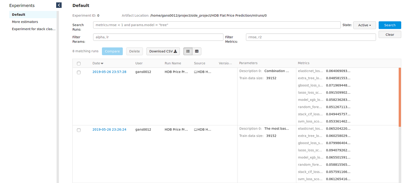
It is a good practice to leave some descriptions regarding any changes or extra processing that you have done in the experiment. This will help you later during the analysis of the result.

Use a smaller sample size for experiment

I learnt this advice from an amazing instructor — Jeremy Howard. He is the founder of fastai, that carries the mission to make AI education free and accessible to anyone.

It is an awesome free online course about machine learning. Do check out their courses if you are interested in getting your hands dirty and kick start your machine learning journey.

So what does this actually mean? In the earlier section, we have explained about the train test split process so that we can get some feedback for our model. Now we can go one step further to create an even smaller sample from our training set, which is meant for experimenting.

Why are we doing this? When we are designing our models or adding new features, we want to get quick feedback from all the activities that we are doing. Waiting 5–10 minutes to experiment on one thing is not going to be productive. Hence, having a smaller sample size, you can run your experiments faster, gain feedback and make changes.

How small the sample size should be? Rules of thumbs — it should be small but representative enough that can help you run your experiment in less than 20 seconds and gain a good rough estimation on the results.

Create our machine learning model

Sklearn provide a lot of handy libraries that help us to create our model easily. You can create multiple models and run all of them in a single experiment, see the code below as an reference :

elasticnet = make_pipeline(RobustScaler(), ElasticNet(alpha =0.00001, random_state=1))

svm = make_pipeline(RobustScaler(),SVR(C=140))

lasso = make_pipeline(RobustScaler(), Lasso(alpha =0.0005, random_state=1))

GBoost = GradientBoostingRegressor(loss='huber',min_samples_split=10,n_estimators=200)

experiment_description = [
 'Add in sale year and sales month feature',
 'Add more data from 2015'
]

run_experiment([elasticnet,svm,lasso,GBoost],experiment_description)

The code might look very minimal, but it requires a great amount of knowledge in understanding the theory behind those models. For instance, you need to know what is the mathematical theory behind the model, what are the hyperparameters, where and when we should use this model.

Each model deserve one whole article to explain the theory and mechanism behind it thoroughly. Look up the resources online, there are a ton of useful materials out there.

Ensemble

This is a very useful techniques in machine learning in boosting up the accuracy of your overall model. What it does is to create a bunch of different classifiers (for instance: random forest, elasticnet, xgboost), and ensemble the results of these classifiers to improve the result.

One simple and common ensemble technique that we could use is simply averaging the prediction of every classifier.

You might be wondering how does it help? The rationale behind is that, different classifier is learning the pattern of the data set from different perspective. By gathering and averaging the results, we could see some performance gain.

Stacking

The ensemble techniques that I am using here is stacking. This is a slightly advanced technique compared to averaging the model. Nevertheless, what it did under the hood is very simple! Below is the simple architecture of stacking:

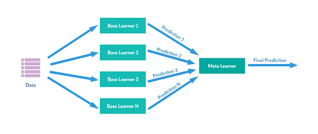
We have multiple classifiers learning on the data and outputting many different predictions. Instead of averaging the predictions, we send it to a meta learner, which is another machine learning model to give us the final prediction.

The meta learner is deciding the weights on the predictions made by the different classifiers. Some classifiers might perform better than the others, so the meta learner will optimize and find the best combination.

As daunting as the whole process may sound, this actually requires a very minimal amount of codes as the heavy lifting is done by our awesome sklearn library !

Metrics

Time to see some results! But first we need to understand what are the metrics before analyzing the result.

The metrics that we are using here is Root Mean Square Logarithmic Error (RMSLE). I believe most of you have heard and learnt Root Mean Square Error (RMSE) before. The difference between these two metrics are we apply log for the target value and the predict value before calculating the root mean square. See the equations below :

Why are we using RMSLE instead of RMSE? By doing log, we are only looking at the relative difference/percentage difference between the real and predicted value.

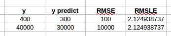
RMSE gives a very big penalization if the difference between the target value and predict value is numerically big. But RMSLE is looking at the percentage difference and give the same amount of loss score for both cases.

In our project, the price of different flats varies on a different level, we would like all the errors to be treated on a percentage basis, and that is the main reason why RMSLE is used.

Results

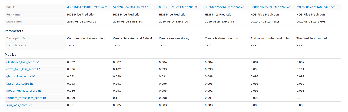
The lower the loss score, the lower the difference between the target and predicted value, hence means better result. From the comparison above, we can know, among all the feature creations, creating the mapping of flat location to region is the most helpful.

By combining all the extra features that we created, the overall improvement is quite significant. You can compare the result between the first column and last column to observe the improvement of the loss score.

The data size that we use for performing all these experiments is only a very small subset of the data. We can run a full experiment (Using all the train data) and compare ‘The most basic model’ — Model A and ‘The model with all the extra features’ — Model B, to verify that our feature creation is actually helpful. See the results below:

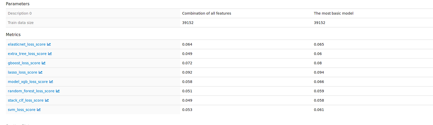
Model B are performing much better across all the models that we are using. So feature creation definitely helps a lot !

I would like to highlight the best performing model among these two, which is the stacking classifier. The stacking classifier of the Model B is having a loss score 15% lower than Model A, which is an amazing improvement.

Conclusion

In a nutshell, I have pretty much highlight the whole process of building a flat price predictor from scratch. You can download the source code from this GitHub repository.

Besides of the machine learning code, I have also created a web application to perform real time prediction.

The web application code is in the same repository and you can refer to them if you find it useful for your use case.